A18 - Basic Video Processing

For all my past blog posts, I have done numerous tasks such as classification, playing musical notes, measuring areas, cleaning by Fourier transform, etc.

But what's the common thing about them? Yes, all of them are based on extracting features using an image only. So the question is, how about videos? Can the same techniques be employed?

In this blog post, I will show you a simple experiment on extracting features from a kinematic event captured using a video camera.

A17 - Neural Networks

Artificial neural network or simply neural network is a mathematical model that aims to mimic the structural/functional aspect of biological neural networks. So what is the difference between the two? Biological networks aim to explain a complex phenomena using real neurons, forming a circuit, releasing physical signals (voltage action potential)to one another. Artificial neural networks, on the other hand, are purely mathematical and uses artificial neurons instead.

A16 - Probabilistic Classification

Pattern recognition has been an interest of many people in the previous years. Many classification tools have been developed to perform this complex task.

In relation to my previous blog post about pattern recognition using the minimum distance classification, I will show you another tool using Linear Discriminant Analysis which is the process of finding a linear combination of features enabling separation of two or more classes of objects [2].

A15 - Pattern Recognition

Humans have an intrinsic capability to differentiate things from each other. That is to recognize an unknown object and classify the group it belongs by just looking at patterns such as color, shape, size, texture, etc. The amazing thing is, we do this complex task in just a short period of time. Not so long ago, computers arrived in the playing field to at least mimic this impressive feat of humans. Computers' do this by doing an inspection on an object's characteristics repeatedly. But for a computer to be able to do this, humans must teach it first. The question is how?

The first important thing a computer must define is a set of object features or pattern. These features are quantifiable properties such as color and size. These features are then used to create classifiers to conveniently group together objects into a class sharing common properties.

In this blog post, I'll show you how to extract features from objects and finally use them to create a function that will do pattern recognition.

A14 - Color Image Segmentation

In today's era, a wide selection of "high-technology" imaging tools have come to life. One can choose from the sleek point-and-shoot cameras, to the high resolution DSLR's and the compact built-in high megapixel cellphone cameras. With all these complicated and expensive tools, we only have one simple ultimate goal. It is just to capture a scene or an important moment in our lives. A pretty simple idea right?

The images we capture can always be separated into two parts, the scene or object of our interest and the background. Sometimes the background is not as interesting as the object/scene but we have no choice but to take them also. That's where image segmentation enters. We can use this method to separate the object from the not-so-interesting background. If you have been following my blog, separating a region of interest (ROI) from the background is not a new idea. And it was always done using grayscale images. But many objects have intrinsic colors similar to the background, thus doing segmentation in grayscale world will definitely fail. In this blog post, I'll show you two techniques, the parametric and non-parametric segmentation, of separating a colored image from a background.

A13 - Image Compression

Remember the old school floppy disk? The unattractive bulky square-like storage device. Imagine this, the device only stores up to a maximum of 1.5 MB only! But it was ubiquitous many years ago that everyone was so contented with it until the arrival of new storage devices with storage size ranging from GB to TB.

With such small storage space, what can we do to maximize its usage??
--> Compression is the answer!

Compressing a file such as a document or an image means reducing its storage size for convenience purposes.

In this blog post, we will use the Principal Component Analysis to represent an image as a superposition of weighted basis images and minimize the number of features to be used to compress the image. A possible useful discussion of Principal Component Analysis method can be found in this wiki page.

A12 - Preprocessing Text

Just some random thoughts... One of the very first things we learned when we started going to school was to write. Writing is a representation of a language through the use of a set of symbols (in our case, alphabet). Before computers became popular, most people hand-write texts, letters, etc.; and the nature of the hand-written text is unique for each individual.

With this concept, how do people understand other people's handwritten text especially if it's too "ugly"?
--> I guess it's our innate ability to read words not letter by letter but by the first and last letters only and decipher the exact word instantly.

In relation to the handwritten text I was talking about above, I'll show in this blog post how to extract handwritten text from an imaged document with lines.

A11 - Playing notes by image processing

Listening to music is an integral part of my everyday life. It relaxes me and gives me my private moment.

Artists and musicians play the music we hear using a score sheet. A sheet with musical notes serving as a guide to perform a piece of music. So how do they play the music derived from a score sheet? A common answer would be via an instrument/voice.

But do you know that we can actually play a music using image processing? Cool!

In this blog post, we will extract musical notes from a digitized score sheet and play these in Scilab with the proper frequency and duration.

A10 - Binary Operations

In connection to my previous blog post on Morphological Operations, I will discuss the techniques involved in Binary Operations. As what you can infer from the name, it is all about operations involving binarization of an image.

Why and where is this technique useful then? Why binarize the image in the first place?

--> The answer is simple, binarizing an image makes it easier to separate the region of interest (ROI) from a background. If the separation is successful, we can then perform many processes in understanding the ROI. For example, in medical imaging, cancerous cells are often larger than normal cells, thus we can easily detect and separate them from the background and from normal cells by applying binary operations. Reading through this blog post will give you an idea on the procedure of this technique.

A9 - Morphological Operation

Today, we'll all talk about shapes... shapes... shapes...

When I hear the word morphology, the first thing that comes to my mind is the biological context related to the study of structures and forms of plants and animals. Basically, this instinctive definition of mine can be stretched out to the image processing context. Practically, it means the same thing but instead of organisms, we talk about anything with no life like shapes.

Moving one step forward, morphological operations are then operations on an image that transform it to another for further processing and information extraction. These operations apply a structuring element (sort of a basis image) to an input image, creating an output image of the same size as the structuring element.

The most common type of morphological operations are dilation and erosion.

A8 - Enhancement in the Frequency Domain

Today is July 21, 2011 -- exactly 5 weeks after I put up this blog... It was fun writing notes and nerdy stuff here knowing the fact that anybody, anywhere around the globe, can actually reach and read this blog. Amazing huh!

Anyway, going back to what this post really is about, I will show you how to enhance an image by removing or improving some parts in the frequency domain. To be able to follow the concepts I will use in this post, you must have some background in using Fourier Transform, if not, you can visit first my previous posts here and here.

The basic idea of this post is that whenever we have an image with repetitive patterns which are not necessary, we can get its Fourier Transform. By doing so, we are now in the frequency domain so we can create a filter that will remove frequencies pertaining to the unwanted patterns. And viola! The unwanted patterns are gone!

A7 - Properties of the 2D Fourier Transform

This time around, I would be talking about something you guys are familiar with already, FOURIER TRANSFORM. But just in case it's the first time you visit my blog, I suggest you read through first 2 days old post about Fourier Transform here.


With the use of my good friend Scilab, I'll show you what happen to different patterns when operated by Fourier Transform (FT). Recall that we can directly get the Fourier Transform in Scilab by using the function fft2() and shifting its quadrants using fftshift(). (Remember to take the absolute value first using abs() before shifting.)

The patterns I used here are 128x128 images of square, annulus, square annulus, two symmetric slits along the x-axis and two symmetric dots along the x-axis. Results are shown below

Figure 1. (A) square (B) annulus (C) square annulus (D) two symmetric slits

(E) two symmetric dots (F-J) Corresponding FT of A to E

Just in case you wonder what the FT really looks like because the pattern produced is not really obvious, we can play a trick by creating smaller versions of A to E (not image size wise) and take their FT's.

Figure 2. (A) square (B) annulus (C) square annulus (D) two symmetric slits

(E) two symmetric dots (F-J) Corresponding FT of A to E

Now that looks clearer now. Figure 1 and 2 provides us a small bank of the Fourier Transform of some common basic patterns observable in real life optical systems. These correspondences are often called Fourier Transform (FT) pairs. Oftenly, it is helpful and saves time to know the FT pair of common patterns beforehand instead of deriving each everytime you need it.

We now proceed to the anamorphic property of Fourier Transform. Anarmophic according  to [2] is the production of an optical effect along mutually perpendicular radii. Basically, we'll talk about the FT of sinusoids and the corresponding modifications to it when we try distorting the sinusoids. 

As a start, let's observe the FT of a simple sinusoid with varying frequency of the form z = sin(2*pi*f*x). 

 

Figure 3. (A-F) Sinusoids of frequency 2, 4, 6, 8, 10 and 20 Hz.

(G-L) Complementary FT of A to F.

We can see that the FT of a sinusoid produces two identical peaks symmetric about the center of the image and along the axis of the sinusoid. This is indeed true since FT decomposes a signal to its consequent frequencies. Thus, the two peaks represent two frequencies for a sinusoid which are equal and just negation of each other. On the other hand, we can observe that as the frequency of the sinusoid increases, the peaks move upward/downward. This is because the derived component frequencies go higher and moves further away from the center.

If we try adding a constant bias to a sinusoid or technically shifting its value to the positive region, the outcome is

 

Figure 4. (A) Sinusoid of frequency 4Hz with 

added constant bias of 1. (B) FT of A.

In figure 4B, we notice another peak present in the center of the image (try clicking the image to enlarge). The reason for the center peak is that another component was separated by FT with 0 Hz frequency corresponding to the added constant bias. This is factual because a sinusoid (sine) with 0 frequency is a constant. This observation can be useful in finding actual frequencies in interferograms with DC biases. Just remove the 0 frequency peak and the observed frequencies will then be correct.

Suppose however a non-constant bias(another sinusoid with low frequency) is added, what happens to the FT? 

Figure 5. (A) Sinusoid of frequency 4Hz with 

added 0.5Hz sinusoid bias. (B) FT of A.

Looking at figure 5, we can still apply the same reasoning of removing the peaks very close to 0 to get the actual frequencies of an interferogram.

We further move one step higher by rotating our sinusoid with respect to different angles. Just change the sinusoid to the form

theta_deg = 30;
theta = theta_deg*(%pi/180);
z = sin(2*%pi*f*(y*sin(theta) + x*cos(theta)));

Note: The conversion of theta_deg to theta is necessary because the argument supported by Scilab trigonometric functions is radians. 

 

Figure 6. (A-F) Sinusoids of frequency 4Hz rotated by 30, 60, 

90, 120, 150 and 180 degrees. (G-L) FT's of A to F.

We can observe that as the rotation angle increases, the peaks move counterclockwise about an angle equal to the rotation angle. The important artifact to remember is that the rotation did not change the presence of two frequencies as observed in figure 3H. The FT simply rotated as a result of the rotation of the sinusoid.

If we are then to create a sinusoid as a result of multiplication of two perpendicular sinusoids,

 z = sin(2*%pi*4*x).*sin(2*%pi*4*y);

the following result happens

 

Figure 7. (A) Sinusoid as a result to multiplication of 4Hz 

sinusoids along x and y. (B) FT of A.

The result shown in figure 7B suggests that the peak frequencies doubled instead of the usual two and they went off the center axes. The doubling phenomena happened because the two frequencies corresponding for each sinusoid along a certain position paired up. In particular, the observed peaks correspond to combinations of 4 and -4Hz along the x-direction with the 4 and -4Hz along the y-direction. The locations would then be at (4,4), (4,-4), (-4,4) and (-4,-4).

As curiosity-driven people, we can try combining the sinusoid described in figure 7A with one rotated sinusoid as shown

 

Figure 8. (A-G) Figure 7A with added single rotated 

sinusoid with angles 0, 30, 60, 90,120, 150, 180 

degrees respectively.

A good prediction would be that the FT will four frequencies as shown in figure 7B can still be seen with additional frequencies rotated. Basically, just integrate figure 7B with figures 6G-6L individually.

 

Figure 9. (A-G) FT of figures 8A-G, respectively.

Aha! We had a correct prediction! What if we try to incorporate 6 sinusoids rotated an angle 30, 60, 90, 120, 150, and 180 at the same time to figure 7A. I must say that the resulting FT should look like a superposition of figures 9B-G. And since the chosen angles somewhat form half of a full rotation, I think the FT would have a circle in the middle.

Figure 10. (A) Combination of 1 multiplication of two perpendicular

sinusoids and 6 rotated sinusoids. (B) FT of A.

Indeed, the formed pattern has a circle inside!! 

In conclusion, this activity was pretty much a good one for understanding Fourier Transform deeper. The key idea is that whenever we combine sinusoids and produce complicated patterns, the Fourier Transform decomposes the frequencies we used to provide a clearer picture on the operations we used to create the pattern.

For this activity, I would give myself a grade of 10.0 for producing all the outputs necessary and for giving clear figures that explains the objectives.

References:

[1] 'Properties of the 2D Fourier Transform', 2010 Applied Physics 186 manual by Dr. Maricor Soriano

[2] http://www.thefreedictionary.com/anamorphic

A6 - Fourier Transform Model of Image Formation

If you would ask a physicist some terms or concepts commonly used in his/her field, Fourier Transform may have a good chance coming out. You know, Fourier Transform may sound so creepy to guys doing something far from physics, but it's just a piece of mathematical tool that does great wonder =)

Fourier transform decomposes a signal into its component frequencies. It has a wide range of application, from optics to signal and image processing and to real life devices such as spectroscopy to magnetic resonance imaging [2].

In strict mathematical definition, the Fourier Transform(FT) of an two dimensional image f(x,y) is

Equation 1. Fourier transform

where fx and fy are the component frequencies along x and y. However, if you don't have a background in programming, you would ask how to implement equation 1 numerically. The answer would be to discretized equation 1 in the form

Equation 2. Discrete Fourier Transform

where xo and yo are spatial intervals between consecutive signal samples in the x and y [3]. In most programming software, the implementation is called a Fast Fourier Transform (FFT). In Scilab, the function is fft2().

The output of the FFT is a complex number array where the diagonals of its quadrant interchanged as shown below

Figure 1. Quadrant conversion from image to FFT output.

 To see what fft2 in Scilab can do, we apply it to a 128x128 image of a white circle and letter "A".

Figure 2. (A) binary image of a circle. (B) circle FFT. (C) circle shifted FFT. 

(D) circle inverse FFT. (E) binary image of "A". (F) "A" FFT. 

(G) "A" shifted FFT. (H) "A" inverse FFT.

Figures 2A and 2E are the images of a circle and letter "A" created using Scilab and Paint. We then use the fft2() of Scilab to get the Fourier transform of these images as shown in 2B and 2F. However, since the output of an FFT is a complex array, we must take its intensity value instead using abs(). 

Taking note of the quadrant shifting described in figure 1, the results of 2B and 2F must be shifted back to original quadrant orientation using  fftshift(). The results can be seen at figures 2C and 2G and it can be noted that 2C is actually verifying the analytical Fourier Transform of a circle. To check whether the obtained FFT results are correct, an inverse FFT is done by taking the FFT of the results of 2C and 2G. The corresponding results are shown in 2D and 2H which are obviously (well for letter "A") inverted. 

Now, after familiarizing ourselves with FFT, we now move one step higher by introducing my friend Mr. Convolution. Convolution practically is just a combination of two functions producing a modified version of the two. Mathematically speaking, it is expressed as 

 

Equation 3. Convolution integral

We now take use of this beautiful convolution integral by simulating an imaging device. Yes, an imaging device! Suppose you have a camera or something that has a lens in it, if you try covering parts of the lens, what effects do you observe in the image output? Hmmm... Verify your intuition by reading further.

So we create a 128x28 image of the letters "VIP" filling up approximately 50% of the space (figure 3) and a white circle same as in figure 2A. The letters will serve as our image to be captured and the circle as our aperture. 

 Figure 3. Created "VIP" image.

We can implement equation 3 by first taking the FFT fft2() of figure 3 and fftshift() of figure 2A. To get the convolved image, we get the inverse of the product of their FFT. If we do this for circles of different radii, the results will be as follow

 

Figure 4. (A-E) Circular apertures of radii 0.1, 0.3, 0.5, 0.7 and 0.9.

(F-J) Convolved images corresponding to apertures in A to E.

We may observe that the resulting images are inverted as compared to the original image figure 3. And as the aperture's radii decreases, the images' resolution decreases as well becoming "blurrier". This is practically true in real life as less light enters the device and thus producing low quality image.

After saying hi to Mr. Convolution, I want you to meet Mr. Correlation. From the word's English definition, correlation is indeed the measure of similarity between two objects or in our case two functions. If you're interested with its mathematical expression, it is 

Equation 4. Correlation function p.

At first glance, it pretty looks like the same as the convolution integral, but it's not. The only chance they become equal is that when f and g are even functions. cool!

But where do we use Mr. Correlation? --> We can use it for pattern recognition or template matching. I'll tell you how.

We first create a 128x128 image of a text "THE RAIN IN SPAIN STAYS MAINLY IN THE PLAIN." We will try to recreate this text using 128x128 image of the letter "A" with the same font and font size as with the text. We then take the inverse FFT of the product of the FFT of "A" and the conjugate of the FFT of the text. In Scilab, the easier way to take a conjugate is by using conj(). If you got a bit confused, a snippet of the code is output = fft2(Fa.*(conj(Ftext))) where Fa is the FFT of "A" and Ftext is the FFT of the text. Results are

  

Figure 5. (A) Text. (B) letter "A". (C) output. (D) shifted FFT of C.

It can be seen in figure 5D that the text is somewhat mimic to some extent. Locations of letter "A" produced the highest correlation translating to a brighter image which indeed brought the idea that correlation can be actually used in finding words in a document.

Another template matching application is edge detection where the edge pattern is matched with an image. We can implement this by making a 3x3 matrix of an edge pattern where a value of negative -1 can be treated as an edge. (NOTE: total sum must be zero!). In Scilab we can create different edge patterns such as horizontal, vertical, diagonal and spot by using the matrices

pattern_hor = [-1 -1 -1; 2 2 2; -1 -1 -1];

pattern_ver = [-1 2 -1; -1 2 -1; -1 2 -1];

pattern_diag = [-1 -1 2; -1 2 -1; 2 -1 -1];

pattern_spot = [-1 -1 -1; -1 8 -1; -1 -1 -1];

These pattern matrices are convolved with the VIP image as in figure 3 using the Scilab function imcorrcoef(grayscale image, pattern). Results are shown below.

Figure 6. (A) horizontal pattern. (B) vertical pattern. (C) diagonal pattern.

(D) spot pattern. (E-H) Convolved image of VIP with A-D.

We can see from the results of figure 6, the resulting convolved image follows the edges feed into them. Horizontal pattern makes the horizontal edges of VIP more pronounced while vertical pattern highlights the vertical edges. The spot pattern in turn created the clearest edge detection result due to the fact that it somewhat combines the horizontal and vertical patterns.

Woohoo! This was a fun activity, I learned a lot... I already have thoughts of applying the methods in my future works. 

I would probably give myself a grade of 10.0 for producing all the outputs needed in this activity and producing good figures to back my results.

References:
[1] 'Fourier Transform Model of Image Formation', 2010 Applied Physics 186 manual by Dr. Maricor Soriano
[2] http://en.wikipedia.org/wiki/Fourier_transform#Applications
[3] http://fourier.eng.hmc.edu/e101/lectures/Image_Processing/node6.html

A5 - Enhancement by Histogram Manipulation

Image is an imitation of the form of an object, place or a person. Appreciation towards images is often proportional to the extent of its quality. However, quality may be affected by many different factors such as lighting, camera resolution, type of focus method, to name a few.

So how do we improve the quality of an image without repeating image acquisition?

--->> The answer is through histogram manipulation.

An image histogram provides us a quick look on the tonal distribution of an image. We can then enhance the quality or certain features of an image by manipulating its pixel value. I'll show you how to do this in this blog post.

First, we obtain from our collection a picture/image that seems to be dark in its nature.

 

Figure 1. Image to be enhanced. 

(image taken from http://baisically.blogspot.com/2011/01/sad-panda-8.html)

We convert the image into grayscale mode and take its histogram. We then obtain the cumulative distribution function(CDF) from the probability distribution function(PDF) or the normalized histogram. In Scilab, this can be done by using the cumulative sum function cumsum(x) where x is a matrix or vector. In simple terms, CDF is the probability that a value will be found less than or equal to an x value.

 Figure 2. Enhancement preliminaries. (a) Grayscale conversion of figure 1.

(b) Grayscale histogram of figure 1. (c) CDF of normalized version of (b).

We do the enhancement by backprojecting the image pixel values to the pixel value of our desired CDF. For example, our desired CDF is a straight increasing line.

Figure 3. Backprojecting method.

We take a grayscale value of x1 and find its CDF value y1. We then trace y1 in the desired CDF as y2. After tracing y1 to y2, we get the corresponding grayscale value x2 of y2. Finally, we replace x1 by x2 in the image concerned. We repeat the process for all grayscale values from 0-255 of our original CDF.

Since we now know the backprojecting method, we create different desired normalized CDF's of linear and nonlinear form.

 

Figure 4. Different desired CDF's. (a) Linear. (b) Quadratic. (c) Cubic.

(d) Gaussian. (e) Logarithmic. (f) Hyperbolic tangent

The CDF's are acquired using the code snippet below:

grayscale = 0:255;

cdf_linear = (1/255)*grayscale;   //linear CDF
cdf_quadratic = ((1/255)*grayscale).^2;   //quadratic CDF
cdf_cubic = ((1/255)*grayscale).^3;    //cubic CDF

a_gauss = 0.01; b_gauss = -((1/255)^2)*log(100);
cdf_gaussian = a_gauss*exp(-b_gauss*grayscale.^2);   //gaussian CDF  Note: cdf value from 0.01 to 1.

a_ln = (exp(1)-1)/255; b_ln = 1;
cdf_ln = log(a_ln*grayscale + b_ln);    //logarithmic CDF 

b_tanh = atanh(-0.99); a_tanh = (1/255)*(atanh(0.99)-b_tanh);
cdf_tanh = (tanh(a_tanh*grayscale + b_tanh))/1.98 + 0.5;     //hyperbolic tangent CDF

To get the corresponding new grayscale values of 0:255 depending on the desired CDF, we invert the equations of our desired CDF's which in turn makes the CDF values of our original image (cdf_original) as our independent variable. You can follow the code snippet below.

grayscale_linear = round(255*cdf_original);
grayscale_quadratic = round(255*sqrt(cdf_original));
grayscale_cubic = round(nthroot((255^3)*cdf_original, 3));
grayscale_gaussian = round(sqrt(-log(cdf_original/a_gauss)/b_gauss));
grayscale_ln = round((exp(cdf_original)-b_ln)/a_ln);
grayscale_tanh = round(1/a_tanh*(atanh(1.98*(cdf_original-0.5))-b_tanh));

After applying the method as described above, the resulting modified images are

 

Figure 5. Modified images based from a CDF of (a) linear, (b) quadratic,

(c) cubic, (d) gaussian, (e) logarithmic and (f) hyperbolic tangent.

To be able to verify whether the modified images have the desired CDF, we take their corresponding normalized histograms(or pdf) and get their CDF.

Figure 6. Histograms based on the CDF type of (a) linear, (b) quadratic,

 (c) cubic, (d) gaussian, (e) logarithmic and (f) hyperbolic tangent.

Figure 7. Retrieved CDF of modified images based on the CDF type of 

(a) linear, (b) quadratic, (c) cubic, (d) gaussian, (e) logarithmic and (f) hyperbolic tangent.

Looking at figures 4 and figures 7, we can say that the CDF's are exactly the same suggesting that the backprojecting method is indeed effective.

Now, we comment on the alteration of the original image according to a particular CDF.

• For a linear CDF, the image became brighter and seems to be equalized.
• For a quadratic CDF, the image is brighter as compared to using a linear CDF.
• For a cubic CDF, the image is even brighter as compared to both the linear and quadratic CDF.
• For a pseudo-gaussian CDF, the image became very bright insinuating image overexposure.
• For a logarithmic CDF, the image is similar to when using a linear CDF with only slight increment in the presence of almost black colors.
• For a hyperbolic tangent CDF, the image became grayish since the histogram shows that more values can be found in the gray region.

The procedure above is coded personally using a programming language, however there are available freewares online that do histogram manipulation. One of the common freeware is GNU Image Manipulation Program (GIMP). A copy of which can be found here. GIMP is a very powerful image processing software comparable to Adobe photoshop.

In GIMP, histogram manipulation can be made by first opening your desired image. You can then convert this into grayscale by clicking the Image button and choosing Grayscale in the Mode selection. To automatically graph the histogram of the grayscaled version of your image, click Colors and choose Curves. To start histogram manipulation, just drag the diagonal straight line in the Curves window and observe the changes in the image at the main window. Snapshots of different diagonal line orientations are shown below.

Figure 8. Sample histogram manipulation in GIMP.

 Figure 9. Another sample histogram manipulation using GIMP.

That's it! You can choose whatever CDF you want depending on what effect you would want to happen on your image. Enjoy image enhancement  in the future!

As a conclusion, I would give myself a grade of 10.0 for completing the activity and producing all required output, for providing good figures with complete units and captions, and for taking the initiative of implementing the method on 5 different nonlinear CDF's.

References:

[1] 'Enhancement by Histogram Manipulation', 2010 Applied Physics 186 manual by Dr. Maricor Soriano

A4 - Area Estimation for Images with Defined Edges

Was there a point in your life wherein you asked yourself how the government measures land area? How about scientists' way of estimating the size of cells?

Yes, one possible way is to do these tasks manually. However, manual calculation of areas/sizes often induce time conflicts.So the last resort is to create a program that will automatically do these tasks...

In this blog post, I will teach you how to estimate areas of shapes with defined edges using the technique derived from the Green's theorem.

Haha, I can hear you mumble and puzzled on how to use Green's theorem.

Strictly speaking, Green's theorem relates the line integral around a closed curve to a double integral over a region bounded by the closed curve with mathematical expression

Equation 1. Green's theorem 

where F1 and F2 are continuous functions.

In physics or mathematics, we often consider double integral as a representation of a region's area.

The summarized equations related are as follow:

• We first consider a bounded region R.

 

Figure 1. Region R with a counterclockwise contour.

• Choosing F1=0, F2=x, equation (1) becomes                                     

 

Equation 2.

•  We next choose F1 to be -y and F2 to be 0, then equation (1) becomes

 Equation 3.

• Then the area of region R is just the average of the right hand sides of equations (2) & (3).    

 

Equation 4.

• Finally, if there are Nb pixels in the boundary, we can discretize equation (4) as

Equation 5.

Equation 5 will be the basic equation we will use in all parts of this post.

The next task is to implement equation (5) to obtain area estimations of shapes with defined edges and check the extent of its accuracy as compared to the theoretical areas of the shapes. The task will be easier if you create a black and white geometric shape such as a rectangle, a square, a circle, etc. If you need help on how to create these kind of black and white shapes, you can first read my blog post here.

In this post, I will show you the implementation of the technique on a square and a circle.

We first create circles of different radii along a 1000x1000 pixel area and save them in bmp format. The equivalent of this on a physical sense is a 2x2 sq. unit area. The radii I will use are 0.1, 0.2, 0.3, 0.4, 0.5, 0.6, 0.7, 0.8, 0.9 and 1.0 units.

Figure 2. Circles with increasing radii.

To obtain the x and y values we will use in equation (5), we implement a function in Scilab 4.1.2  follow(Img). This function returns two lists x and y which are points in the contour of the area concerned. The resulting plots using these x and y are

Figure 3. Contours of the circles in figure 2.

There are two ways of obtaining an estimation of the areas of the circles. 

First, we take the sum of the pixel values of the image using sum(I). This is plausible since the corresponding matrix of a binary image contain only values of 1 and 0. Thus, if we take the same sum of all the pixel values, we are in a way taking the total pixel values of a region where the area is our concern.

Second, we will use Green's theorem and the derived equation (5). 

A summarized version of the code is shown below

I = imread(image);  //opening an image

[x,y] = follow(I);   //parametric contour

scale_factor = 2/1000;   //scale conversion 1000x1000 pixel = 2x2 region
xi = x'*scale_factor;     //rescaling pixel value to physical value

yi = y'*scale_factor;    //rescaling pixel value to physical value

xi_1 = [xi(length(x)), xi(1:length(x)-1)];

yi_1 = [yi(length(y)), yi(1:length(y)-1)];
  

theoretical_area(i) = %pi * (radius^2);    //theoretical area

sum_area(i) = sum(I) * (scale_factor^2);    //area using the sum method

greens_area(i) = abs(0.5*sum(xi.*yi_1 - yi.*xi_1));    //area using the Green's method

The results and the corresponding percent errors are shown in table 1 and the plot of the errors for both the sum method and the Green's method is shown in figure 4.

Table 1. Results for circles of different radius on a 1000x1000 pixel area

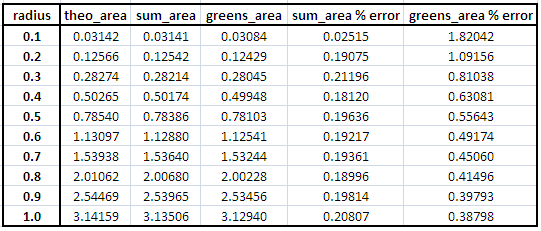
Figure 4. Plot of % errors of area estimation using sum and Green's theorem methods.

We can see that the sum method is more accurate than the Green's theorem method. We can also notice that as we increase the radius of the circle, the error decreases for the Green's theorem method while the sum method produces an almost non-changing error(except for r=0.1). The apparent error using Green's theorem method may be attributed to the fact that the pixels along the edge(contour) is not included in the area's computation. Also, the area of a circle contains an irrational number pi which is very difficult to approximate.

We must also take note that if we're talking about small numbers, small deviations or differences will result to large percent errors.

We apply the same method for squares of varying side lengths of 0.1, 0.2, 0.4, 0.6, 0.8, 1.0, 1.2, 1.4, 1.6 and 1.8. Results are shown below

 

Figure 5. Squares with increasing side length and has a 1000x1000 pixel area

Table 2. Results for squares of different side length 

 

 Figure 6. Plot of % errors of area estimation using sum and Green's theorem methods.

The same conclusions are achieved as that of circles. However, this time the sum method produced 0% error for any side length.

We emphasize that in the above method, I used an image of 1000x1000 pixel area. What if we decrease the pixel area size? Will there be a significant difference in the result? Since the main purpose of this activity is to investigate how well the Green's theorem method approximate areas. We probe this in the next part of this blog post. 

We follow the same method as above while changing the total pixel size area to 100x100, 200x200, 300x300, 400x400, 500x500, 600x600, 700x700, 800x800, 900x900 and 1000x1000. The resulting contour plots for both circle and square are

 

Figure 7. Contours of circles of varying pixel area size and constant radius = 0.5

Figure 8. Contours of squares of varying pixel area size and constant side length = 0.8

We then plot the %errors achieved by the Green's theorem method

Figure 9. Plot of % errors of area estimation of a circle using Green's theorem methods.

Figure 10. Plot of % errors of area estimation of a square using Green's theorem methods.

For both cases, we can safely conclude that as the resolution of the shape decreases, the error increases. This is due to the fact that for low resolution shapes, the contours are not continuous. You can actually verify this by enlarging(clicking) figures 7 and 8.

Now we know how to estimate areas of given shapes, we implement our technique in estimating the area of an actual location in the Philippines.

I particularly choose the University of Sto. Tomas, a very close university to my heart and my house. According here, the UST campus has a land area of 21.5 hectares or 2314240 sq. ft. or 215000 sq. m. The goal is to estimate the land area of UST using the methods above and compare it with the actual land area.

Figure 11. Map of UST obtained using Google map.

Using Gimp 2.0, I cropped figure 11 to a smaller pixel size area  and highlighted the area of interest.

                 

Figure 12. Cropped version of figure 11.    Figure 13. UST area is highlighted

We then convert figure 13 to a binary image and plot the contour of the edge of the region of interest.

 

Figure 14. Binary form of figure 13.

Figure 15. Contour of the region of interest.

If we apply both sum method and Green's theorem method, the resulting computed areas are 38547 sq. pixels and 38524 sq. pixels. However, these values are in pixel scale, so we have to find a relationship between pixels and actual physical units. The way to do this is to go back to figure 11. Google map provides us a scale of the map at the lower left portion. 

Figure 16.Actual scale.

So we count the number of pixels corresponding to 500ft. and 200m. The same method as in my previous blog post is used. I found out that 66 pixels = 500 ft and 87 pixels = 200 m. Using these conversion factors, we now observe the accuracy of our method.

Table 3. Results for the estimation of UST's land area.

We can see that approximately the error for the sum method is between 4% to 6%; and for the Green's theorem method, the error is approximately between 5% to 6%. This simply means that the method implemented above are good to some extent.


After 16 figures, 3 tables and 5 equations, I now conclude that this post is done! Hurrah!

Overall, I would give myself a grade of 10.0 for implementing the Green's theorem method in estimating areas of shapes with defined edges, for implementing another method of taking the sum of the pixel values of the binary images, for noting the accuracy of the methods for different parameters such as length of region and pixel area size, and for finding a way of using the given methods in estimating the area of a real world location.

 References:
[1] 'Area estimation of images with defined edges', 2010 Applied Physics 186 manual by Dr. Maricor Soriano
[2] http://www.symbianize.com/showthread.php?t=425263
[3] Google maps