A1 - Digital Scanning

Today, technology has improved a lot that almost any tool imaginable is accessible. (Thank God I am a 90's baby =)... However, during the medieval period (well just an exaggeration), people don't have access to computers with sophisticated graphing tools. Remember that graphs are vital and are the most read part of a scientific article.

So how do scientific knowledge propagate then?

Aha! Yes, we're thinking the same thing! They hand-draw graphs! A very difficult task indeed because manual graphing are more prone to errors which may lead to ambiguous data and misconception.

So the first activity for my Applied Physics 186 class is digital scanning, that is our objective was to scan a hand-drawn graph and try to reconstruct this using the most famous Microsoft Excel. The hand-drawn graph I used was taken from the thesis manuscript entitled "Relaxation times and the initial conditions of the one-dimensional Fokker-Planck equation" by Josefino Z. Villanueva on September 1973.

Figure 1. Scanned hand-drawn graph.

Procedure:

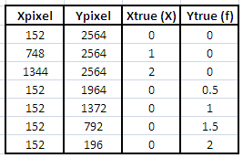
I first used GIMP 2.0 to rotate the scanned graph since the x axis is not parallel to the lower edge. I did this by using the Measure tool which uses two assigned points to measure the required tilting angle. After rotating, the pixel coordinates of the origin and the visible tick marks along the x and y axes are located to be able to formulate an equation to convert pixel coordinates to physical coordinates. The obtained pixel coordinates of the tick marks and their corresponding physical values are

Table 1. Pixel coordinates and their physical values along x and y.

Then, I plot the Physical Value along x (Xtrue) versus Pixel coordinate along x (Xpixel) to obtain a best fit line which will be the basis conversion equation to get physical values along x from pixel coordinates along x for the entire activity. The same has been done for Ytrue and Ypixel. The obtained best fit lines are Xtrue = 0.00168*Xpixel - 0.25503 and Ytrue = -0.00085*Ypixel + 2.16584.

          Figure 2. Best fit line of Xtrue versus Xpixel.      

 Figure 3. Best fit line of Ytrue versus Ypixel.

Since I now have conversion equations, I proceed to obtaining pixel coordinates of the data points for one of the curves in figure 1 and replicate figure 1 by using the formulated equations for conversions. The obtained digital plot is

Figure 4. Digital plot of the scanned graph.

To verify whether the digital plot is indeed right, I overlayed a cropped version of figure 1 to figure 4 and see if the two corresponding curves superimpose. This is easily done by right clicking the plot in Microsoft Excel and select Format Chart Area. In the Fill section, select Picture or text fill and click File. Choose the image you want and adjust it to your desire by changing the percent values in the Fill > Offsets section.

Figure 5. Digital plot overlayed with a cropped version of figure 1.

Looking at figure 5, we may say that the digital conversion(blue markers and line) of the hand-drawn curve is good, if not excellent, because only little parts of the original hand-drawn curve is visible.

To be able to make sure that the algorithm and process is really good, I digitally converted all other curves available in figure 1(shown in figure 6) and overlayed the cropped version of figure 1(shown in figure 7).

Figure 6. Digital conversion of the entire curves in figure 1.

Figure 7. Digitally reconstructed graph overlayed with the original graph.

By looking at figure 7, the process is indeed successful in converting a hand-drawn plot to a digital version. Small deviations in the digital conversion may be associated to the difficulty of pointing the exact pixel coordinates of the curves in the graph.

However, for this activity I give myself 10 points for the successful correspondence between the scanned graph and the digital conversion of one curve in the graph and for completing the all parts of this activity. And probably give myself a bonus of 2 points for taking the initiative of testing the process in digitally converting two other curves present in the scanned graph.

I would like to thank Dr. Soriano for the useful hints and insights for this activity and Tracy for getting the hand-drawn graph from the NIP library and scanning it.