Yes, one possible way is to do these tasks manually. However, manual calculation of areas/sizes often induce time conflicts.So the last resort is to create a program that will automatically do these tasks...
In this blog post, I will teach you how to estimate areas of shapes with defined edges using the technique derived from the Green's theorem.
Strictly speaking, Green's theorem relates the line integral around a closed curve to a double integral over a region bounded by the closed curve with mathematical expression

Equation 1. Green's theorem
where F1 and F2 are continuous functions.
In physics or mathematics, we often consider double integral as a representation of a region's area.The summarized equations related are as follow:
- We first consider a bounded region R.

Figure 1. Region R with a counterclockwise contour.
- Choosing F1=0, F2=x, equation (1) becomes

Equation 2.
- We next choose F1 to be -y and F2 to be 0, then equation (1) becomes

Equation 3.
- Then the area of region R is just the average of the right hand sides of equations (2) & (3).

Equation 4.
- Finally, if there are Nb pixels in the boundary, we can discretize equation (4) as

Equation 5.
Equation 5 will be the basic equation we will use in all parts of this post.
The next task is to implement equation (5) to obtain area estimations of shapes with defined edges and check the extent of its accuracy as compared to the theoretical areas of the shapes. The task will be easier if you create a black and white geometric shape such as a rectangle, a square, a circle, etc. If you need help on how to create these kind of black and white shapes, you can first read my blog post here.
In this post, I will show you the implementation of the technique on a square and a circle.
We first create circles of different radii along a 1000x1000 pixel area and save them in bmp format. The equivalent of this on a physical sense is a 2x2 sq. unit area. The radii I will use are 0.1, 0.2, 0.3, 0.4, 0.5, 0.6, 0.7, 0.8, 0.9 and 1.0 units.

Figure 2. Circles with increasing radii.
To obtain the x and y values we will use in equation (5), we implement a function in Scilab 4.1.2 follow(Img). This function returns two lists x and y which are points in the contour of the area concerned. The resulting plots using these x and y are

Figure 3. Contours of the circles in figure 2.
There are two ways of obtaining an estimation of the areas of the circles.
First, we take the sum of the pixel values of the image using sum(I). This is plausible since the corresponding matrix of a binary image contain only values of 1 and 0. Thus, if we take the same sum of all the pixel values, we are in a way taking the total pixel values of a region where the area is our concern.
Second, we will use Green's theorem and the derived equation (5).
A summarized version of the code is shown below
I = imread(image); //opening an image
[x,y] = follow(I); //parametric contour
scale_factor = 2/1000; //scale conversion 1000x1000 pixel = 2x2 region
xi = x'*scale_factor; //rescaling pixel value to physical value
xi = x'*scale_factor; //rescaling pixel value to physical value
yi = y'*scale_factor; //rescaling pixel value to physical value
xi_1 = [xi(length(x)), xi(1:length(x)-1)];
yi_1 = [yi(length(y)), yi(1:length(y)-1)];
theoretical_area(i) = %pi * (radius^2); //theoretical area
sum_area(i) = sum(I) * (scale_factor^2); //area using the sum method
greens_area(i) = abs(0.5*sum(xi.*yi_1 - yi.*xi_1)); //area using the Green's method
The results and the corresponding percent errors are shown in table 1 and the plot of the errors for both the sum method and the Green's method is shown in figure 4.
Table 1. Results for circles of different radius on a 1000x1000 pixel area
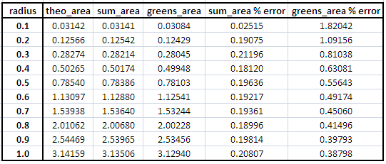

Figure 4. Plot of % errors of area estimation using sum and Green's theorem methods.
We can see that the sum method is more accurate than the Green's theorem method. We can also notice that as we increase the radius of the circle, the error decreases for the Green's theorem method while the sum method produces an almost non-changing error(except for r=0.1). The apparent error using Green's theorem method may be attributed to the fact that the pixels along the edge(contour) is not included in the area's computation. Also, the area of a circle contains an irrational number pi which is very difficult to approximate.
We must also take note that if we're talking about small numbers, small deviations or differences will result to large percent errors.
We apply the same method for squares of varying side lengths of 0.1, 0.2, 0.4, 0.6, 0.8, 1.0, 1.2, 1.4, 1.6 and 1.8. Results are shown below

Figure 5. Squares with increasing side length and has a 1000x1000 pixel area
Table 2. Results for squares of different side length


Figure 6. Plot of % errors of area estimation using sum and Green's theorem methods.
The same conclusions are achieved as that of circles. However, this time the sum method produced 0% error for any side length.
We emphasize that in the above method, I used an image of 1000x1000 pixel area. What if we decrease the pixel area size? Will there be a significant difference in the result? Since the main purpose of this activity is to investigate how well the Green's theorem method approximate areas. We probe this in the next part of this blog post.
We follow the same method as above while changing the total pixel size area to 100x100, 200x200, 300x300, 400x400, 500x500, 600x600, 700x700, 800x800, 900x900 and 1000x1000. The resulting contour plots for both circle and square are
Figure 7. Contours of circles of varying pixel area size and constant radius = 0.5
Figure 8. Contours of squares of varying pixel area size and constant side length = 0.8
We then plot the %errors achieved by the Green's theorem method

Figure 9. Plot of % errors of area estimation of a circle using Green's theorem methods.

Figure 10. Plot of % errors of area estimation of a square using Green's theorem methods.
For both cases, we can safely conclude that as the resolution of the shape decreases, the error increases. This is due to the fact that for low resolution shapes, the contours are not continuous. You can actually verify this by enlarging(clicking) figures 7 and 8.
Now we know how to estimate areas of given shapes, we implement our technique in estimating the area of an actual location in the Philippines.
I particularly choose the University of Sto. Tomas, a very close university to my heart and my house. According here, the UST campus has a land area of 21.5 hectares or 2314240 sq. ft. or 215000 sq. m. The goal is to estimate the land area of UST using the methods above and compare it with the actual land area.

Figure 11. Map of UST obtained using Google map.
Using Gimp 2.0, I cropped figure 11 to a smaller pixel size area and highlighted the area of interest.


Figure 12. Cropped version of figure 11. Figure 13. UST area is highlighted
We then convert figure 13 to a binary image and plot the contour of the edge of the region of interest.

Figure 14. Binary form of figure 13.

Figure 15. Contour of the region of interest.
If we apply both sum method and Green's theorem method, the resulting computed areas are 38547 sq. pixels and 38524 sq. pixels. However, these values are in pixel scale, so we have to find a relationship between pixels and actual physical units. The way to do this is to go back to figure 11. Google map provides us a scale of the map at the lower left portion.

Figure 16.Actual scale.
So we count the number of pixels corresponding to 500ft. and 200m. The same method as in my previous blog post is used. I found out that 66 pixels = 500 ft and 87 pixels = 200 m. Using these conversion factors, we now observe the accuracy of our method.
Table 3. Results for the estimation of UST's land area.

We can see that approximately the error for the sum method is between 4% to 6%; and for the Green's theorem method, the error is approximately between 5% to 6%. This simply means that the method implemented above are good to some extent.
After 16 figures, 3 tables and 5 equations, I now conclude that this post is done! Hurrah!
Overall, I would give myself a grade of 10.0 for implementing the Green's theorem method in estimating areas of shapes with defined edges, for implementing another method of taking the sum of the pixel values of the binary images, for noting the accuracy of the methods for different parameters such as length of region and pixel area size, and for finding a way of using the given methods in estimating the area of a real world location.
References:
[1] 'Area estimation of images with defined edges', 2010 Applied Physics 186 manual by Dr. Maricor Soriano
[2] http://www.symbianize.com/showthread.php?t=425263
[3] Google maps
No comments:
Post a Comment